Inclusive Analysis of Gender Diversity Among Data Scientists
Abdul Majed Raja recently wrote a nice post analyzing gender diversity within the Kaggle Survey data. This survey, which ran from August 7th to August 25th of 2017, was an “industry-wide survey to establish a comprehensive view of the state of data science and machine learning” with data from 16,716 participants.
Here, I extend Abdul’s work to include responses from participants who did not identify as male or female. This is not a critique of the initial work. I have certainly carried out analyses where I’ve excluded the analysis to males and females. However, with 16K+ respondents, I figured this would be a dataset where non-binary individuals could be included. So, I decided to pick up where Abdul left off. As such, I’ve tried to keep the graphs in the same aesthetic as his original post.
Additionally, this work holds the same disclaimer as Abdul’s original post. This dataset certainly is subject to selection bias and is not necessarily representative of all data science practitioners. Nevertheless, when data are there, it is important to look at the data and draw reasonable conclusions with these limitations in mind.
#Loading Required Libraries
library(dplyr)
library(stringr)
library(ggplot2)
library(ggthemes)
library(tidyr)
library(scales)

## Download data here
## Login required
# https://www.kaggle.com/kaggle/kaggle-survey-2017?

#Load Input Data
complete_data <- read.csv("../kaggle-survey-2017/multipleChoiceResponses.csv",header = T, stringsAsFactors = F)
Gender across Data Science
From Abdul’s original post, I noticed that there was a nonzero number of non-binary respondents.
# Gender distribtuion chart - borrowed from original post (just slightly increased font size)
complete_data %>%
  filter(GenderSelect!='') %>%
  group_by(GenderSelect) %>%
  count() %>%
  ggplot(aes(x = GenderSelect,y = (n / sum(n))*100))+
  geom_bar(stat = 'identity') + ylab('Percent') +
  theme_solarized() +
  scale_x_discrete(labels = wrap_format(10))+
  theme(axis.text = element_text(size = 20), axis.text.x = element_text(angle = 0, vjust = 0.5, hjust = 0.5), axis.title=element_text(size=20)) +
  ggtitle('Gender Distribution of Kaggle Survey Respondents')

This is where my analysis diverges from Abdul’s. I got curious as to what the gender breakdown analysis would look like indvidiuals who identified as “A different identity” or “Non-binary, genderqueer, or gender non-conforming” included.*
## With many respondents, we don't have to restrict to male and female respondents
complete_data %>%
  filter(GenderSelect %in% c('A different identity','Non-binary, genderqueer, or gender non-conforming')) %>%
  group_by(GenderSelect) %>%
  summarise(count = n())
The data include 159 individuals who identify as “A different identity” and 74 who identify as “Non-binary, genderqueer, or gender non-conforming.”
To get a better understanding of how people specifically responded to the gender question, I took a look at the free form responses.
free_data <- read.csv("../kaggle-survey-2017/freeformResponses.csv", header = T, stringsAsFactors = F)
## there are 134 free form responses
free_data %>% filter(GenderFreeForm!='') %>% dim()
unique(free_data$GenderFreeForm) %>% length
table(free_data$GenderFreeForm) %>% names
Across the entire data set, there were 134 participants who responded to the free form gender question. Among these, there were 104 unique responses.
Among these responses, it became pretty clear that these were individuals who fell into a few general categories:
- people whose gender identity did not fit into the categories “female”, “male,” or “nonbinary, genderqueer or gender non-conforming” (i.e. “Bisexual trans nonconformist”, or “Trans female”, or “transhuman”)
- at least 23 people who identify as some sort of apache/attack helicopter
- a number of respondents who have conflated “biological sex” and “gender”** (i.e. “There are two genders: MALE/FEMALE. I am sorry, but as I scientist I cannot change reality to make people feel good. I refuse to participate in surveys that deny science.” )
- people who identify as male or female (free response was some capitalization variant on “male” or “female”) and entered this into the free form box
- Some other animal (i.e. “Dolphin”, “kitten”) or response (“Jedi”, “Vulcano”, “wtf”, “space marine”, etc.)
This suggests that (1) most non-binary and non-cisgender individuals identified as “nonbinary, genderqueer or gender non-conforming”, “male”, or “female” rather than “A different identity” and (2) a gender-inclusive analysis stratified by country and programming language could render some interesting and informative results about the non-binary community among data scientists.
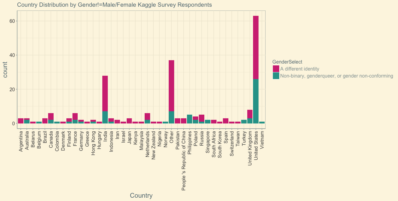
## Country non-binary respondents
complete_data %>%
  filter(GenderSelect %in% c('A different identity','Non-binary, genderqueer, or gender non-conforming'), Country != '') %>%
  group_by(Country,GenderSelect) %>%
  summarise(count = n()) %>%
  arrange(desc(count)) %>% ggplot() +
  geom_bar(aes(Country,count, fill = GenderSelect), stat = 'identity') +
  scale_fill_manual(values=c("#d33682","#2aa198"))+
  theme_solarized() +
  theme(axis.text = element_text(size = 12),
        axis.title=element_text(size=16),
        axis.text.x = element_text(angle = 90, vjust = 0.5, hjust = 1),
        legend.text=element_text(size=12)) +
  ggtitle('Country Distribution by Gender!=Male/Female Kaggle Survey Respondents')
Gender by Country
When we look at country, it is clear that these non-binary individuals are contributing to the community all over the world.
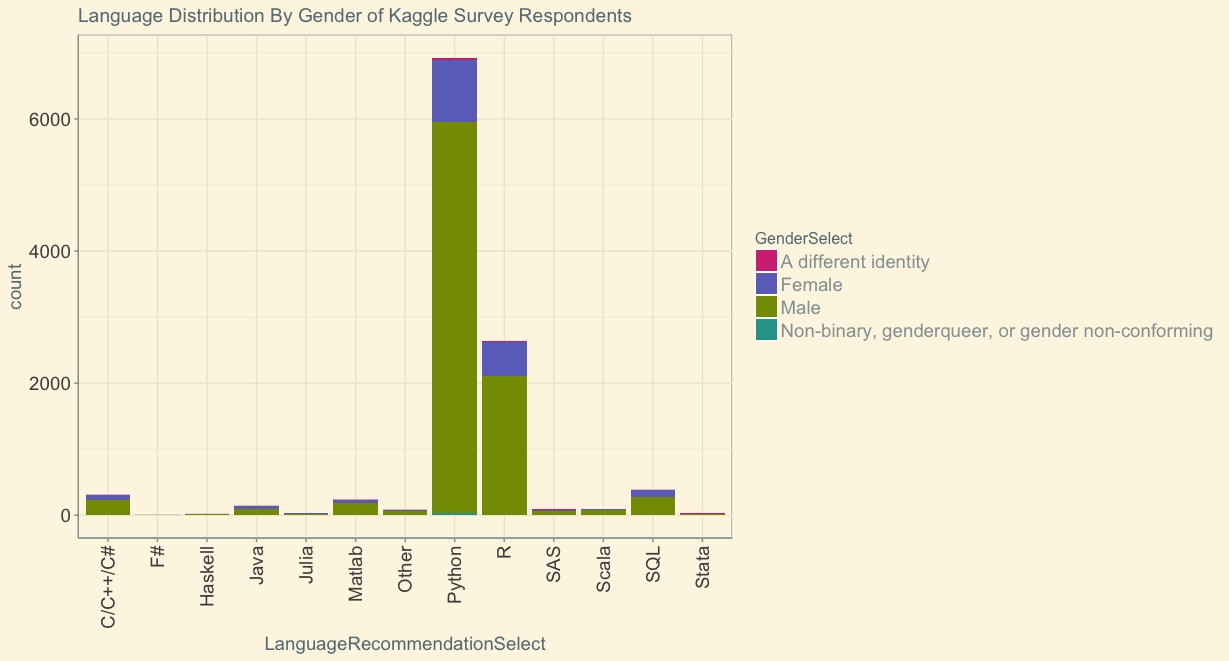
Gender by Programming Language
When we look at the entire gender distribution broken down by programming language, we recapitulate previous findings that Python and R are the top two languages used by data scientists. It also appears that more non-binary individuals may use these two languages.
## Language full gender distribution
complete_data %>%
  filter(GenderSelect!='',LanguageRecommendationSelect!='') %>%
  group_by(LanguageRecommendationSelect,GenderSelect) %>%
  summarise(count = n()) %>%
  arrange(desc(count)) %>% ggplot() +
  geom_bar(aes(LanguageRecommendationSelect,count, fill = GenderSelect), stat = 'identity') +
  theme_solarized() +
  scale_fill_manual(values=c("#d33682","#6c71c4","#859900","#2aa198"))+
  theme(axis.text = element_text(size = 14),
        axis.text.x = element_text(angle = 90, vjust = 0.5, hjust = 1),
        axis.title=element_text(size=14),
        legend.text=element_text(size=14)) +
  ggtitle('Language Distribution By Gender of Kaggle Survey Respondents')
## Proportional breakdown by language
complete_data %>%
  filter(GenderSelect!='',LanguageRecommendationSelect!='') %>%
  group_by(LanguageRecommendationSelect) %>%
  mutate(countT=n()) %>%
  group_by(LanguageRecommendationSelect,GenderSelect) %>%
  mutate(count = n()) %>%
  mutate(prop=count/sum(countT)) %>%
  arrange(desc(count)) %>% ggplot() +
  geom_bar(aes(LanguageRecommendationSelect,prop, fill = GenderSelect), stat = 'identity') +
  theme_solarized() +
  scale_fill_manual(values=c("#d33682","#6c71c4","#859900","#2aa198"))+
  theme(axis.text = element_text(size = 16),
        axis.text.x = element_text(angle = 90, vjust = 0.5, hjust = 1),
        axis.title=element_text(size=16),
        legend.text=element_text(size=14)) +
  ggtitle('Proportional Language Distribution by Gender of Kaggle Survey Respondents')
However, when we look at the proportional breakdown scaling for the number of individuals using each language, these data suggest that F# may be the language of choice for Non-binary, genderqueer, or gender non-conforming individuals. However, looking at the previous plot, this is reflective of the small sample size of F# users (N=4).

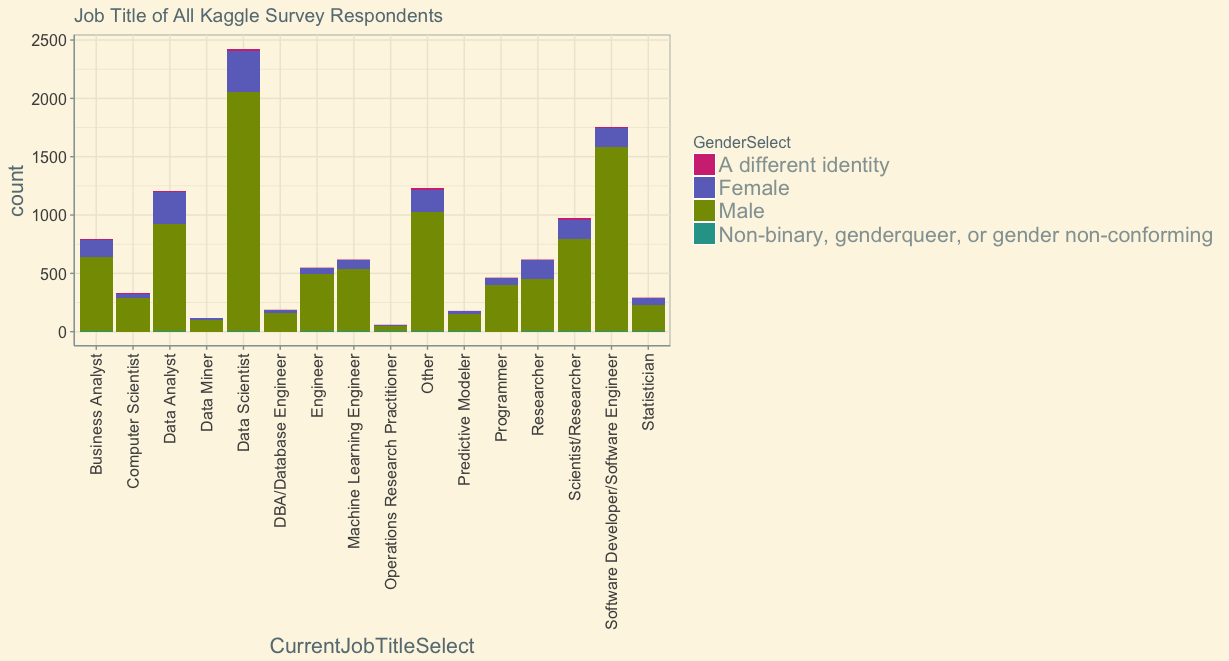
Gender by Job Title
As reported previously, survey participants most frequently hold the job title of “Data Scientist.”
## what about job title?
complete_data %>%
  filter(GenderSelect!='',CurrentJobTitleSelect!='') %>%
  group_by(CurrentJobTitleSelect,GenderSelect) %>%
  summarise(count = n()) %>%
  arrange(desc(count)) %>% ggplot() +
  geom_bar(aes(CurrentJobTitleSelect,count, fill = GenderSelect), stat = 'identity') +
  #facet_grid(.~GenderSelect)  +
  theme_solarized() +
  scale_fill_manual(values=c("#d33682","#6c71c4","#859900","#2aa198"))+
  theme(axis.text = element_text(size = 12),
        axis.text.x = element_text(angle = 90, vjust = 0.5, hjust = 1),
        axis.title=element_text(size=16),
        legend.text=element_text(size=16))+
  ggtitle('Job Title of All Kaggle Survey Respondents')
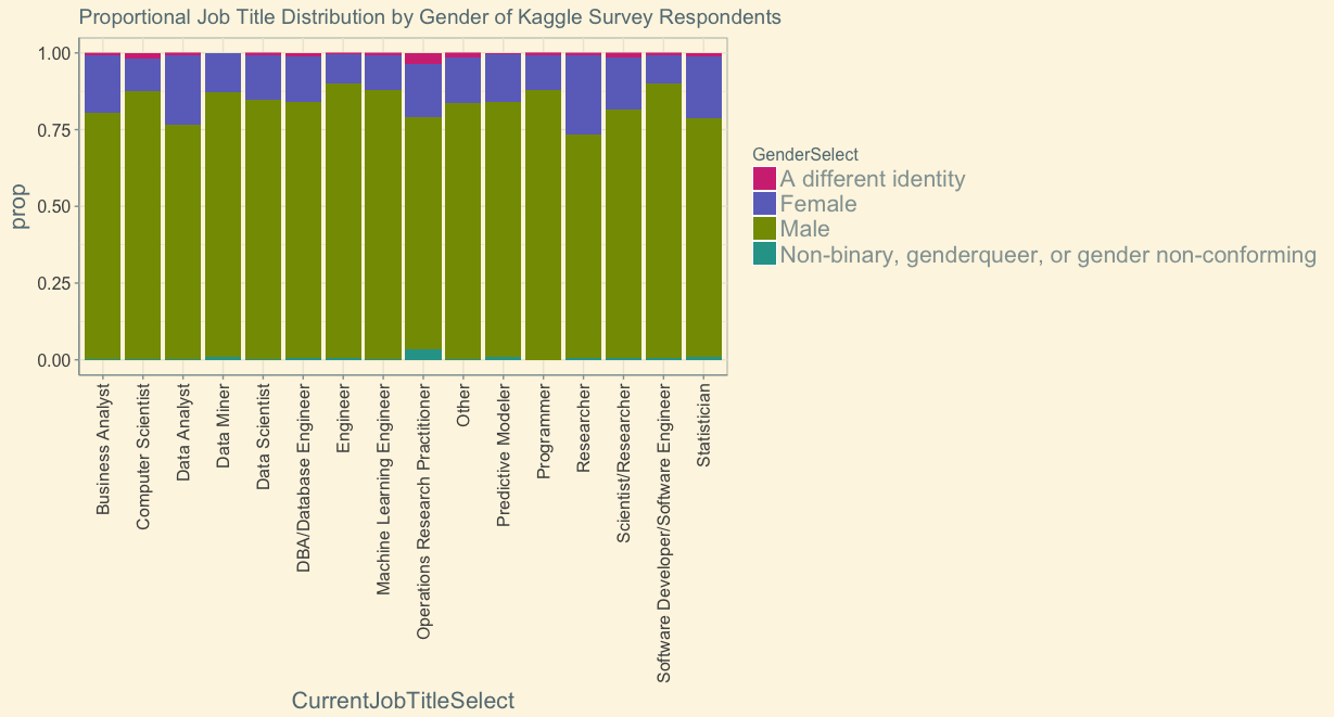
If we normalize for the number of participants in each job title, it appears that there are more non-binary individuals with the job title of “Operations Research Practitioner.” However, this again reflects the small number of participants in this job (N=57 across all genders). Regardless, this plot demonstrates that non-binary individuals contribute across all job titles.
## proportional job title
complete_data %>%
  filter(GenderSelect!='',CurrentJobTitleSelect!='') %>%
  group_by(CurrentJobTitleSelect) %>%
  mutate(countT=n()) %>%
  group_by(CurrentJobTitleSelect,GenderSelect) %>%
  mutate(count = n()) %>%
  mutate(prop=count/sum(countT)) %>%
  arrange(desc(count)) %>% ggplot() +
  geom_bar(aes(CurrentJobTitleSelect,prop, fill = GenderSelect), stat = 'identity') +
  #facet_grid(.~GenderSelect)  +
  theme_solarized() +
  scale_fill_manual(values=c("#d33682","#6c71c4","#859900","#2aa198"))+
  theme(axis.text = element_text(size = 12),
        axis.text.x = element_text(angle = 90, vjust = 0.5, hjust = 1),
        axis.title=element_text(size=16),
        legend.text=element_text(size=16)) +
  ggtitle('Proportional Job Title Distribution by Gender of Kaggle Survey Respondents')
Conclusions
The good news is that individuals across the gender spectrum are now able to more accurately identify in survey data. In fact, a 2015 survey to examine the experiences of transgender people in the United States had responses from 27,715 people. However, in data science, as is often the case generally, the conclusions we can draw are limited due to small sample sizes. This suggests that working to be more inclusive as a community will help improve the accuracy of analyses of this type. More importantly, however, improved inclusivity will improve diversity of background and ideas within the field improving the field as a whole.
Notes
*In my original post I used the term ‘non-cisgender’ throughout; however as Sharla Galfand graciously pointed out Twitter, many non-cis individuals, such as trans men and women, would have identified as either male or female, as that is their gender! I have changed the language throughout this post to refer to non-binary individuals when appropriate, rather than using the term non-cisgender. Thank you, Sharla!
**Biological sex can be defined as ‘male’ or ‘female’ and relates to the chromosomes in your cell. Gender is a social construct that is well-explained here with a glossary of terms here.